Identifying Risk Using ODC Based Growth Models

Ram Chillarege and Shriram Biyani
IBM TJ Watson Research Center, Yorktown Heights, NY, 1994

Published: Fifth IEEE International Symposium on Software Reliability Engineering, November 1994, Monterey, CA - IEEE Computer Society. Copyright, IEEE.

Introduction

Growth modelling, to understand an aspect of software reliability, has several challenges in its use. The published work indicates that there is substantial understanding of its use in the late system test and early field life [8] [10] [4] [3] including the practical aspects of real life data [5]. We also recognize that the use of this as an evaluation tool, does not remove the responsibility of trying to get a better handle of identifying guidelines to improve the process [7]. Our observation, in the practical use of these methods in real development, is that they are usually more successful either in late system test or early field life rather than during the function component test and early system test. Thus, there is a view from the development manager, that professes, that it is rather late in the cycle to realistically do anything significant to correct process problems [2].

Ideally, if reliability growth modelling could be used earlier in the development process, it could provide greater feedback to the management. It is not that it cannot be used - it is just hard. The type of information that can be gleaned from the models is not much better than the use of defect discovery rates that are quite commonly used to determine staffing of testers and fixers. Thus, when there is an increase in the discovery rate beyond nominal values, it kicks off a war room process to determine re-staffing levels and exposures in the ship dates. The question is: can reliability growth models do more than signal alerts - i.e. provide guidance?

This paper proposes a technique that combines Orthogonal Defect Classification (ODC) with growth modelling to provide far greater insight than is commonly available using typical growth models. There are two elements to this insight. One, contributed directly from ODC and the other in combining the relative growth of different groups of defects and projecting them on a common abscissa to make qualitative inferences.

To illustrate these ideas, section 2 of this paper briefly describes ideas of ODC, relevant to the theme of the paper and section 3 describes the qualitative aspects of a typical growth curve. This is done from experience having seen the growth curves developed for several shipped products. Section 4 combines ODC and Growth Modelling and exploits the relative growth to provide causal insight and means to assess risk. Section 5 illustrates these ideas with data from the real world and section 6 provides a summary. This paper should be of interest to the practitioner as well as the theorist, since it opens up a new dimension to measure progress, while there is still an opportunity to take actions and correct the product and process.

Background on ODC

This paper draws from several ideas of Orthogonal Defect Classification (ODC) and combines them with traditional growth modelling. In this section we will briefly review some of the background on ODC pertinent to the discussion and completeness of the paper. A more detailed discussion on the subject can be found in [1].

ODC originally stemmed from the findings, that different types of defects demonstrate fairly radical differences in their growth models [2]. The study showed that when defects were uniquely categorized by a set of defect types, representing the semantics of the fix, it was possible to relate changes in the shape of the reliability growth curve to defects of a specific type. This was exploited to develop a categorization scheme such that the categorized information from a defect provided measurements on the process. ODC requires that the categorization be orthogonal in the value set for an attribute, so that, as the product moves through the process, the distribution of the values change, explaining the progress of the product.

There is a set of necessary and sufficient conditions that makes a classification, defined by attributes and value selections, ODC. This has to do primarily with its capability to explain the progress of a product through the process, using categorical data, extracted from the defects. Fundamentally, the initial research work demonstrated that semantic information from defects, suitably extracted through classification, could provide insight into the progress of the product, [2]. Next, clever techniques to extract this were developed, providing fairly sensitive instruments to measure progress [1]. ODC is currently practiced in several products spread across 12 IBM locations worldwide. Four attributes - defect type, trigger, impact, and source - are added to the existing data captured by IBM defect tracking tools. These data provide a multidimensional view into the development process, and since the carefully designed classification is architected to provide a measurement, they open numerous opportunities for detailed analysis. Contrasted with root-cause analysis, which tells a developer many details on a few specific problems, ODC provides a view of the total phenomenon occurring over a larger population of defects. For this paper, we will be taking advantage of one of the attributes called defect type. The defect type distribution is designed so that its distribution changes as the product progresses through the process. The signature that the distribution generates, provides a far more sensitive instrument than other purely numeric techniques, to gauge the progress of the product. Since we will be using the value set of the defect type attribute in this paper, we will review some of its details.

A programmer making the correction usually chooses the defect type. The defect type signifies the meaning of the eventual correction. These types are simple in that they should be obvious to a programmer, without much room for confusion. In each case a distinction is made between something missing or something incorrect. A function error is one that affects significant capability, end-user interfaces, product interfaces, interface with hardware architecture, or global data structure(s) and should require a formal design change. Conversely, an assignment error indicates a few lines of code, such as the initialization of control blocks or data structure. Interface corresponds to errors interacting with other components, modules or device drivers via macros, call statements, control blocks or parameter lists. Checking addresses program logic which has failed to properly validate data and values before they are used. Timing/serialization errors are those which are corrected by improved management of shared and real-time resources. Build/package/merge describe errors that occur because of mistakes in library systems, management of changes, or version control. Documentation errors can affect both publications and maintenance notes. Algorithm errors include efficiency or correctness problems that affect the task and can be fixed by (re)implementing an algorithm or local data structure without the need for requesting a design change.

The defect types are chosen to be general enough to apply to any software development, independent of a specific product. Other defect classification schemes exist, see, for example, [6]. The ODC defect types, however, are by design, strongly associated with the project phase, and are therefore, expected to follow different growth trajectories. Their granularity is such that they apply to any phase of the development process, yet can be associated with a few specific phases in the process. The function and algorithm defects could be discovered and fixed anywhere in the verification process, but reflect design aspects of the development effort. Assignment and Checking signify defects that are more likely to be coding issues than any other activity, whereas interface reflects low level design type work.

  
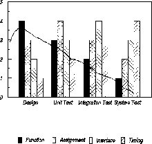
Figure 1: Defect Type Distribution by Phase

Figure 1 is a simplified illustration of the change in defect type distribution as a product moves through different phases. In the design phase, the function errors are most frequent, but their relative contribution drops off in later phases. Assignment errors, reflecting coding issues, increase from design phase to unit test and drop somewhat in the later phases. Interface and timing errors increase peak during the integration test and system test respectively.

In the following sections we will exploit the defect type attribute of the ODC classification on defects, to improve the insight that can be gleaned through growth models. This is done by comparing the relative growth of different types of defects.

Subjective aspects of Growth Curves

Before combining ODC with growth curves, it is important that we discuss, in general, some of the qualitative types of growth curves. Figure 2 shows a typical reliability growth curve with the cumulative number of defects on the ordinate and calendar time on the abscissa. This is one of the fairly standard representations, which will be the one discussed in this paper. There are, however, several variations of these: The ordinate may represent failure rate, and sometimes failure density. The abscissa may represent calendar time, execution time, test cases run, percent of test cases, etc. However, for this paper, we restrict our attention to growth curves with the cumulative number of defects on the ordinate and calendar time on the abscissa. The ideas that are proposed may map into other representations, however, that discussion is not the focus of this paper.

There is a subtlety that is often not discussed in growth models - i.e. what time period is captured in the abscissa of such a representation? We believe it is a very significant part of the discussion, that is often overlooked. It is important for several reasons - the simplest being that the units of measure that are used for the abscissa should have some consistency across all the phases of software development that it spans. For instance, if the abscissa spans, code inspection, unit test, function test and system test, one has to question if days make sense all through that span of the process. If not, there should be some normalization done, so that the measure of reliability on the ordinate makes sense. This question gets deeper, when considering that the work is done by a team and the units should be normalized to reflect either the effort by the team or the coverage of the product. We raise this point to bring to attention that this process is fairly complicated and the answers are not uniformly available. In this paper, we have chosen the span of time from the beginning of the function test until the product is shipped. Based on communication with developers, we believe that this choice provides a reasonably consistent time scale.

The growth curve in Figure 2 is meant to show a span of development periods that begin around the time of the function/component test (FCT), continued into the system test and possibly the early part of the field introduction. The part of the curve which has an accelerated defect detection rate is usually where the function test is ramping up. During FCT not all the code is integrated, but there is probably a substantial amount of parallel testing of the components with the test cases developed, alongside the product. At some time, when most of the test cases have been run, the product is integrated and the system test is begun that starts to stress the code. The ideal time to release the product is after the knee in the curve, which reduces the exposure of defects being found in the field. In practice, several variances occur. Products are not shipped at the knee, as would be ideally desired. The knee can occur in the field. When one does ship just after the knee, there is often another knee that develops a few months out into the field.

  
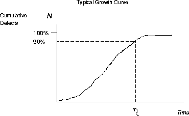
Figure 2: Typical Growth Curve

For the discussion in this paper, we identify one key point on the growth curve, projected on the time line, which is used to compare different growth curves. We find it useful, from practice, to identify the point, when 90% of the predicted total number of defects are found. In the figure, this is annotated as , and referred to, in this paper, as the point. It is intended to approximately represent the knee of the curve. It may or may not be visible depending on how far the growth curve has progressed. When visible, it provides a useful milestone in the development cycle to make comparative assessments.

Combining ODC and Growth Modelling

Separate growth curves can be generated for each of the defect type categories, demonstrating their relative growth. This is not always practical, since some of the categories may be sparse - such as build/package/merge. It is often meaningful to collapse some of the categories, to better reflect a broader aspect of the development process. Function and algorithm defects integrate the design and low level design aspects of the product. Similarly, assignment and checking tend to be related to coding quality. A reasonable collapsing of the categories provides a few useful subdivisions of the data, making the relative comparison far more comprehensible.

  
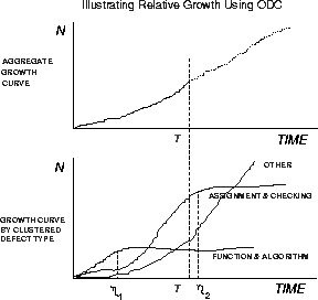
Figure 3: ODC For Risk Assessment

However, when split by three groups of defect types, (shown below) there is much greater insight into what is happening in the development. Here, it is obvious that function and algorithm defects have stabilized, since that growth curve has already reached its knee. This is a sign that the design aspects of the products are stable.

On the other hand, the code quality represented by assignment and checking defects has not stabilized anywhere close to the degree that function defects have. Yet, clearly this growth curve has well passed the inflection point and the knee of the curve is predictable reasonably well, with the existing model. Between the function+algorithm growth curve and the assignment+checking growth curves, it looks as though the code parts of the product will stabilize, a little after the design aspects. The regular testing effort, if continued, should stabilize the product, with respect to the quality of code. On the other hand, this is not so with the third growth curve (miscellaneous or other), which combines user interface, documentation etc. This growth curve is clearly rising very rapidly and the prediction of when it will stabilize is much further out. It is also clear that these miscellaneous defects tend to dominate the overall growth curve in the top half of the figure.

Looking at the relative growth curves, a development manager could respond to what is occurring in the product by carefully choosing the right skill mix and staffing levels during the later parts of testing. It is evident that the lead developers, with the design skills, are not necessarily required at time and they can be moved on to the next release. Whereas, defects of type assignment+checking, representing coding issues, will be opened at current rates, given the testing effort, which will need appropriate skills to close them and staffing to handle the volume. However, the volume is dominated by other defects including documentation and interface problems. There is a major exposure here, since the end is not in sight, and the management has to deal with stabilizing this aspect of the product. Since the type of problems are known, management has the opportunity to respond to it by process changes and bringing the right type of skills and experience to bear. Also, the severity of the defects can be examined, to understand the risk of shipment without complete closure of the open problems.

Real World Example

The data for this example is taken from a large project which used ODC. The defect classification used in this project included an additional category of panels/messages, which is not part of the scheme of [1], where most such defects might be classified as documentation or interface. The time frame includes the function test and the system test up to a couple of months before the desired ship date. Figure 4 shows the overall trend of the cumulative number of defects found during the system test. It appears that the cumulative number of defects is steadily growing and stabilization of the product from the perspective of the growth curve is still far away. The developers perception, during the test effort, is that the product is not yet stable and growth models only re-affirm that belief: that is, the defect discovery rate is high from previous experience. The volume is being handled by increased staffing, but the question of why and what specifically to do, to meet the schedule and to reduce the risk in the field, is not evident from this level of analysis.

  
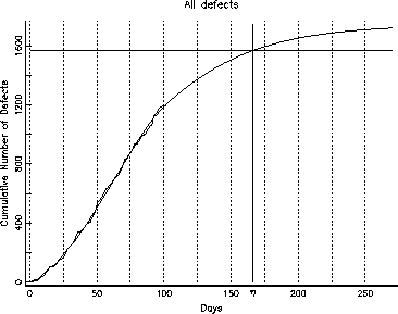
Figure 4: Overall Cumulative Defects

To gain more insight into the data, we used the ODC attribute Defect Type to split the defects into three categories: function defects, assignment+checking and all others termed miscellaneous. The last category predominantly consists of documentation and panel+message defects. Figure 5 shows the separate growth curves for the three categories superimposed on each other. Observe that the defect growth for function and assignment+checking defects is slowing down and both of these categories are expected to stabilize soon. The growth of defects in the miscellaneous category, however, shows no signs of stabilization.

We decided to predict the future course of the growth curve using the Inflection S Curve model [9],

where is the cumulative number of defects found by time t, n is the total number of defects originally present, and and are model parameters related to the defect detection rate and the ratio of masked/detectable defects.

We used the calendar time for t, since it seemed reasonable to assume that, except for short-term fluctuations, this would be a fair measure of test effort. The model itself does not preclude other choices of time scale, such as execution time, but often in practice, the calendar time is the only one available.

  
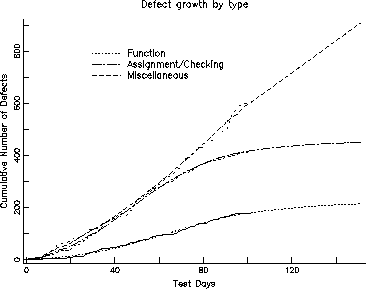
Figure 5: Cumulative Defects by Defect Type

  
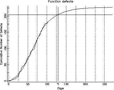
Figure 6: Cumulative Defects: Function

  
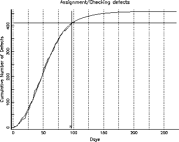
Figure 7: Cumulative Defects: Assignment/Checking

  
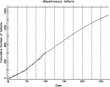
Figure 8: Cumulative Defects: Miscellaneous

We were able to fit the inflection S-curve to each of the first two categories (function and assignment/checking). The growth curve for the other category, however, had not yet reached its knee, and it was not far enough advanced to fit an S-curve to it in the normal manner. We were, however, able to fit an S-curve by assigning a fixed value for one of the parameters , using a guess, based on fitting the model to the entire data. Figures 6, 7 and 8 show the growth curves for the function defects, the assignment and checking defects and the other defects respectively. In each of these curves, there is a horizontal line corresponding to ninety percent of the projected number of defects in this category. The intersection of the horizontal line and the projected growth curve, when projected down to the test phase of the abscissa, will give us the point. For the inflection S-curve, the point is given by:

Notice that the point for function defects is around day 125, and for the assignment and checking is around day 100, but the point for other defects doesn't intercept the projected growth curve all the way past 250 days. Studying these, we can infer that the code quality, represented by assignment+checking defects, in this release is probably stable and is going to stabilize much faster than the function defects. On the other hand, the function defects should stabilize in about a month since we expect to hit the point in about 25 days. The other defects, however, are unlikely to stabilize soon, given the current testing and development activity.

Because of this analysis, comparing the 3 curves, we could say that there is a slight exposure in this product toward the design aspects and much larger one toward the other defects. Therefore maintaining the current test team and development team will probably address the code quality aspects, but one has to aggressively change the process of bringing the skills to address the other two issues. When it comes to function defects, one could argue that the current skill mix, in the development organization, is probably adequate to release the product within the next two months, since the point is only around 25 days away from where we are today. The other defects, however, are the major exposure. The volume of defects in this category outnumber the other kinds of defects and, from our projections, it doesn't look like we have even crossed the halfway point. Therefore, to address this aspect of the product one has to change, not only the skill mix, but also the entire test strategy for these kinds of defects. In a situation such as this, one has to examine the severity distribution of defects under the other category. Commonly, severity is categorized on a scale of 1 to 4 (where 1 is the most severe). Here, it became evident that most of these defects were low severity and potentially a very minor exposure, if any. This knowledge also helps, not only the risk assessment, but also the staffing necessary to address the exposures within a fixed time.

Summary

This paper presents a method to look at the relative growth of defects classified using Orthogonal Defect Classification to gain insight into the behavior of the overall growth curve. This is particularly useful when there is trouble during the development and testing process, identifiable by the overall growth curve, but not providing further insight for management response. Given the pressures in the market, and the speed with which development currently progresses, it is not uncommon that some development efforts find themselves in a difficult position during the latter parts of testing. In such cases, gaining insight into the cause of difficulty is critical for taking the right corrective action.

The contributions of this paper are:

1. Illustrating a method to qualitatively understand the relative growth curve, using a key milestone of a growth curve, which we call the point. Comparing the relative occurrence of the point between growth curves of different defect types, provides insight into the relative rates at which the different aspects of the product are stabilizing.
2. Illustrating the use of this method on a real world example. The example shows a growth curve, where the traditional methods would identify an alarm, without providing any additional insight to deal with the problem. The split of the growth curves, using the ODC defect types, is capable of guiding specific actions to correct the problems.
3. The insight and prediction of the relative growth of specific aspects of the product, identified by the defect type categories, provides a method to evaluate risk. Risk appears in several dimensions. The two more critical ones are schedule and warranty costs. The relative growth models provide the means to determine the skill mix and the staffing levels needed to reduce both risks.

Developers find this a useful method, giving them insight they did not have before. It also provides a reasonable level of quantification to help make better management decisions to significantly impact cost and opportunity.

References

1

CHILLAREGE, R., BHANDARI, I., CHAAR, J., HALLIDAY, M., MOEBUS, D., RAY, B., AND WONG, M. Orthogonal defect classification - a concept for in-process measurement. IEEE Transactions on Software Engineering 18, 11 (Nov 1992), 943-956.

2

CHILLAREGE, R., KAO, W.-L., AND CONDIT, R. G. Defect Type and its Impact on the Growth Curve. In Proceedings of The 13th International Conference on Software Engineering (1991).

3

GOEL, A. L. An Experimental Investigation into Software Reliability. Tech. Rep. TR 88-213, RADC Final Technical Report, 1988.

4

JELINSKI, Z., AND MORANDA, P. B. Software Reliability Research. Statistical Computer Performance Evaluation (1972).

5

KANOUN, K., KAANICHE, M., AND LAPRIE, J. Experience in Software Reliability: From Data Collection to Quantitative Evaluation. Fourth International Symposium on Software Reliability Engineering (1993), 234-245.

6

LLOYD, D. K., AND LIPOW, M. Reliability: Management, Methods and Mathematics. American Society for Quality Control, 1984.

7

MUNSON, J., AND RAVENEL, R. Designing Reliable Software. Fourth International Symposium on Software Reliability Engineering (1993), 45-54.

8

MUSA, J. D., IANNINO, A., AND OKUMOTO, K. Software Reliability - Measurement, Prediction, Application. McGraw-Hill Book Company, 1987.

9

OHBA, M. Software Reliability Analysis Models. IBM Journal of Research and Development 28, 4 (1984), 428-443.

10

RAMAMOORTHY, C. V., AND BASTANI, F. B. Software Reliability - Status and Perspectives. IEEE Transactions on Software Engineering 8, 4 (1982), 354-371.