Ram Chillarege, Kumar Goswami, Murthy Devarakonda CHILLAREGE INC., KOVAIR, IBM, 2002
Abstract: -- A system level fault injection experiment measuring changes in probability of failure and error propagation as a function of failure acceleration. It demonstrates that:
- (1) Probability of failure increases with failure acceleration, and
- (2) Error propagation decreases with failure acceleration.
Published: IEEE International Symposium on Software Reliability Engineering, ISSRE 2002
Introduction
In the past decade fault injection has grown into a research area of its own standing in the dependable computing area. Research in system level fault injection as a means for evaluating and studying systems [Chillarege89, Arlat90] were quickly supported by numerous fault injection platforms to conduct experiments [Barton90, Kanawati95], methods of analysis and experimentation [Gunneflo89, Goswami93, Rosenberg 94] and studies in error propagation [Devarakonda90, Hiller01], and the list goes on and on.
This paper reports on a specific aspect of conducting fault injection experiments, called failure acceleration [Chillarege89]. The concept was proposed at the beginning of the system fault injection era more than ten years ago. This experimental work was done in the late 80s' [Devarakonda90] but remained hidden in a research report succumbing to idiosyncrasies and priorities of an industrial life led by the different authors.
Failure Acceleration provides a theory and means to conduct fault-injection experiments so that the results from such an experiment can be related to probabilities of failure in the real world. Other disciplines of engineering such as mechanical and civil engineering have well developed acceleration methods for reliability measurement. As the area of computer and software engineering matures, and tools such as fault-injection become a regular practice in the discipline, the need for methods of failure acceleration and reliability measurement is felt more strongly. This paper examines the failure acceleration theory, proposed in `89, and provides empirical evidence of its workings.
We believe the results are fundamental, and thus this paper, in spite of the age of this experiment.
Failure Acceleration, Revisited
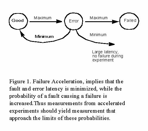
Failure Acceleration is defined by a set of rules that forces fault injection experiments to push the limits of the measurement on the probability of failure.
Figure 1. shows the system in three states, a good state, an error state and a failed state. Concisely failure acceleration is achieved when:
Where p(F) is the probability of a fault causing a failure. The above conditions can be stretched so long as the semantics of the fault model are not altered in the process of altering the controls: namely, the fault injected, and the environment.
In a fault injection experiment, one constructs a fault, injects it into the system and then waits for the system to fail. This would amount to one run of the fault injection experiment. It is not necessary that each of the fault injections cause a failure. Since it is always possible that the error condition created by the injected fault is compensated for, and disappears. On the other hand, the error condition can lay latent for a long time, and not cause a failure during the time allocated for observation in the experiment.
Thus, the measure of probability of failure which is computed after a series of fault injection runs, has factored into it the practices followed in conducting the experiment. How then, do we determine these practices, and relate the results computed from such experiments into real life?
This is why the theory of failure acceleration is important. It gives us a model to construct the experiments, and proposes a way to push the dynamics of the experiment, so that the results from it can be useful and realistic.
Some of the important questions that need to be asked of a fault injection experiment are: what kind of fault does one inject? Is it adequate to inject an error? Once injected, how long does one wait to determine whether or not the system has failed? Since fault injection measurements create censored data, we need to have a means of ensuring that the design of an experiment approaches limits in a predictable fashion.
In Figure 1. it is evident that maximizing the probability of failure involves maximizing the transition into the error state, and the failure state, and minimizing the others. This, plainly is the goal of failure acceleration. The controls in the experiment are primarily the fault which is injected, and the workload environment. They can be varied widely, provided, the fault model used for fault-injection is not compromised.
To achieve acceleration the fault size could be altered, so long as the fault model is not altered. For instance, a large fault can be inserted, which increases the probability of failure, but the size is limited to the extent, say a single fault model does not get distorted to a multiple fault model.
The other control is workload. Increasing the usage in a system decreases error latency in addition to effecting several other system parameters. Managing the workload for acceleration is also much easier, and in this experiment we use this as the primary method to alter acceleration.
When a system is maximally accelerated, the fault and error latencies would be the smallest, and the probability of failure, highest. Then the measurements from the experiment would approach the worst case situation in the field. As a side benefit, the duration of each experimental run would also be shortened. And, consequently the chances of censoring the data prematurely, minimized.
Error propagation is a side effect that can have unpredictable results in the measurements, and therefore is worthy of some discussion and analysis. Error propagation spreads the error state to components that were not intended to be injected to a fault. The main culprit of error propagation is error latency. The longer the system is in error, but working, the error can corrupt system state making the traceability of failure harder. Acceleration shortens error latency, and thereby minimizes the degree of propagation.
In the original work on failure propagation, the system was evaluated using close to maximum acceleration. However, the study itself did not investigate the process of acceleration at different levels, nor study propagation in any detail. Thus, the importance of this experiment and study to investigate the theory.
The Experiment
Fault Models from Field Failure Data
We looked at software errors (severity 1 and 2, on a scale of 1 to 4) from IBM's Virtual Storage Access Method (VSAM) product. VSAM could be considered a file system and a reasonable approximation to what we did not have in terms of failure data on Network File System (NFS). The data covered an aggregate of a few thousand machine years. The study was conducted similarly to the work done by Sullivan, Christmansson and Chillarege [Sullivan91, Christmansson96] which studied failure data from IBM logs. Results of our study revealed that approximately 80% of all faults recorded (regardless of whether they were caused by hardware or software failures) manifest as addressing errors such as incorrect pointers, zero pointers, bad address, overlays and incorrect size and length data. The remaining 20% of the errors were caused by synchronization failures.
We used a packet-based injection scheme which corrupted fields in the NFS packets. The four types of request - Read, Readdir, Create, and Write makeup between 43%-57% of all requests made to an NFS server and represent a close approximation to the various types of addressing errors in our fault mode. Create and Write packets contain pointers to data which can be corrupted to mimic pointer errors and cause overlays. The Read, Readdir, and Write packets contain offset and size fields which can be corrupted to reproduce the remaining types of addressing errors.
We injected errors, that is, corrupted values from the nominal value. By definition, the fault latency is zero, satisfying rule 1 of failure acceleration. The size of the faults varied in displacement sizes from 8 (small), to 256-64000 (medium), and >100,000 (large). The corrupted fields were neither trivial nor unused and helped satisfy rule 3, i.e. increase the probability that the fault injected would cause a failure, thereby reducing the chances of self repair.
Experimental Setup
One has to devise methods to inject the errors, and to monitor critical resources and parameters in the experiment. In this case, it needed kernel support, and utilities to examine the system and application after fault injection. Each of our experiment runs take a while. Often an hour to setup, for cleanup after a failure, re-initialization and getting the workload to the right level. Thus, these system experiments are not fast to run, unlike many of the fault injection experiments that inject programs in a test harness, where thousands of runs can be conducted. Therefore, much thought has been given to the design of the experiment, fault models, injection methods, acceleration, and conducting a matched pair of experiments so the numbers of runs are not too many to gain the insight, and draw the conclusions we need to make.
Since we are also studying error propagation, an additional number of utilities need to be run after the experiment to access whether there was a case of error propagation or not. Thus, the experiments are reasonably elaborate to set up and run.
Matched pair of experiments
A matched pair experiment allows a tighter confidence interval, and reduces the total number of runs in each set to make a binary decision. Each of the matched sets consists of 55 fault injection experiments. The first set is conducted with low load, and the second set with high load. A single fault is injected in each experiment, and the state of the server and client applications is recorded, and separately whether or not there was error propagation which caused the failure. At the conclusion of the runs, the statistics are compared between the two sets of runs.
Acceleration
Acceleration in this particular experiment is achieved through increased workload. We have run this experiment at two settings - one termed low and the other high. The settings were determined by the utilization of server resources (memory, I/O, and CPU). The high workload reflects a system that is just under saturation (i.e. not saturated to the maximum). The low workload is chosen to reflect a system that is busy but can be clearly differentiated from the high case.
Workloads
Each client system participating in the experiment ran a sequential workload that had only one process (one thread of execution) active at a time. At the low load level the server processed 32000 NFS service requests, and at the high load around 72000 requests. The processor utilization ranged 15% - 30% during low load, and 25%-50% during the high load.
The workloads take about 20 minutes to run and the following list illustrates what they are:
- Copying and compiling the source code of a fairly large UNIX command written in C. This workload was created by the Information Technology Center at Carnegie-Mellon University, to compare the performance of remote file systems.
- Building dependencies for object code files for compilation and maintenance of the 4.3BSD UNIX kernel.
- Compiles the 4.3BSD UNIX kernel. Each compilation has 4 stages: macro processor, pass one of the compiler, pass two of the compiler, and the assembler.
- A trace-driven file cache simulation. The trace is read sequentially by the simulation program.
Failure categories
The failures are broadly divided into two categories: server failures and client failures. It is rare that the client crashes, although the programs being run by the client do terminate. When nothing is detected for a period of time in the range of 15-20 minutes, either visibly or through our failure detection scripts, we conclude that there was no failure caused due to the fault injection. The cases that constitute a server or client failure are:
- Server Failure
- Server crash - the system running the NFS server processes has crashed and needs to be rebooted.
- Server bad - the system running the NFS server has not crashed, but it is in such a bad state that it should be rebooted to return it to normal functioning.
- Client Failure
- Client program crash - the program running on a client system has terminated, and therefore client application is incomplete.
- Client program bad - program running on a client system has gone into a bad state and possibly hung. Therefore it cannot complete, or it completes, but with incorrect data.
Error Propagation
Error propagation is defined as a failure in a component or a program that does not directly depend on the one being fault-injected. In this experimental setup an error propagation occurs when:
- The NFS server crashes some time after completely processing the fault injected packet. The fault injected packet creates a latent fault which is triggered by some subsequent request packet.
- The NFS server switches to a bad state after processing a fault injected packet, thereby impacting all the clients.
- An injection in a packet sent by one client causes a failure in another client.
The experiment was instrumented to distinguish among the three types of error propagation. Type 1 is detected by the server recording whether a response to a fault-injected packet is sent back to the client indicating completion of the request. Type 2 is detected from the statistics and performance measures periodically displayed by the systat program. Type 3 is detected from logs that identify which of the client's packets were injected, versus those that failed.
Results
The results of this paper are summarized in two tables that capture the essence of experiments on fault injection and failure acceleration. Table 1 shows the data on failures and failure classes, and Table 2, the data on error propagation.
Failure Acceleration
There is a substantial difference in the fraction of failures reported between low and high acceleration. In this case, the probability of failure went up from 53% to 65%. This drives home the point that increasing acceleration increases the probability of failure. This confirms the theory proposed in the concept of failure acceleration.
These results are important because it tells us not only how systems behave, but also guides us on conducting experiments. The fact that the measured probability of failure is a function of the degree of acceleration in the system is often overlooked by many fault injection experiments. If so, then the interpretation of the results from an experiment cannot be translated meaningfully.
|
Matched Pair experiments, each with 55 runs, at two levels of failure acceleration/load. |
||||
|---|---|---|---|---|
|
Failure Modes |
Low Load: 15-20% CPU Utilization |
High Load: 25%-50% CPU Utilization |
||
|
|
Nos. |
% |
Nos. |
% |
|
Server Failures |
14 |
25.4% |
17 |
30.9% |
|
Client Failures |
15 |
27.2% |
19 |
34.5% |
|
Total Failures |
29 |
52.7% |
36 |
65.5% |
|
No Failures |
26 |
47.3% |
19 |
34.5% |
The theory also suggests that when a system is maximally accelerated, then these measures are likely to reach limits of the system. While our experiment accelerates the failures, we have stopped shy of saturating the system. It will be interesting for future work to examine the saturation process in failure acceleration.
On a related note, it is interesting to compare this maximum probability of failure, with those reported in the first failure acceleration paper of `89. In both cases, the system was just short of saturation and the probabilities of failure were measured in the neighborhood of 60%.
Error Propagation
Table 2 shows the data on error propagation. The data is separated by whether error propagation was noticed in the server or the client. The last two rows show the total number of propagated failures versus the total number of failures. The column showing percentages represents the percentage of failures that were caused due to propagation. It is therefore computed using the total number of failures in the denominator.
That is glaringly obvious is the decrease in error propagation as a consequence of failure acceleration. The fraction of failures that were due to error propagation decreased from 37% to 20%. This takes place while the probability of failure goes up from 52% to 64%. To date, we are not aware of any results that demonstrated this as clearly. It drives home a few important points about failure acceleration and theory.
|
The (%) column represents percent propagation, and is computed as fractions of failures at each level. The experiments are a matched pair of 55 runs each at two levels of acceleration/load. |
||||
|---|---|---|---|---|
|
Error Propagation category, i.e. failures due to propagation |
Low Load: 15-20% CPU Utilization |
High Load: 25%-50% CPU Utilization |
||
|
|
Nos. |
% |
Nos. |
% |
|
Server Propagation |
6 |
20.6% |
6 |
16.6 |
|
Client Propagation |
5 |
17.2% |
1 |
2.7% |
|
Propagation Failures |
11 |
37% |
7 |
20% |
|
Total No. Failures |
29 |
|
36 |
|
The decreasing of propagation makes sense when one recognizes that the increase in acceleration should decrease error latency. With decreased error latency, there is less of a chance for errors to propagate, since the system is exposed for a shorter duration of time.
Without the analysis of what happens to error latency during acceleration, one could otherwise be misguided to believe that the increase in workload may cause propagation to increase which is not the case as evidenced in this experiment.
A not so obvious aspect of acceleration is that in the process of reducing error propagation, we are also forcing the system to react to the injected error closer to the ``single fault model''. In the limit case of zero propagation, the system is reacting to only one instance of the error; a valuable capability for fault-injection evaluation.
Summary
This experiment confirms the theory of failure acceleration, providing measurement and an insight into the fault injection process. The value of this theory is that it gives the experimentalist a clear and systematic method to design experiments, such that empirical results can be projected to limit probabilities of real systems.
Specifically, the contributions are:
- The fault injection experiment confirms the Failure Acceleration theory proposed in 1989.
- The probability of failure increases with failure acceleration.
- Error propagation decreases with acceleration.
Acknowledgements
These experiments were conducted in 1990 when Ram Chillarege, Murthy Devarakonda, Kumar Goswami, Arup Mukherjee, and Mark Sullivan worked at IBM Watson Research. Arup helped with the Unix kernel, NFS, and workload generation. Mark consulted on the formulation of fault models, drawing from his experience in studying faults and failures from field data in IBM systems.
References
[Arlat90] J. Arlat, M. Aguera, L. Amat, Y. Crouzet, J Fabre, J.C. Laprie, E. Martins, and D. Powell, "Fault Injection for Dependability V: A Methodology and Some Applications", IEEE Transactions on Software Engineering, Vol 16., No. 2, 1990.
[Barton90] J.H. Barton, E.W. Czeck, Z. Z. Segall, D.P. Siewiorek, "Fault Injection Experiments Using FIAT", IEEE Transactions on Computers, Vol. 39, No. 4, 1990.
[Chillarege89] R. Chillarege and N. S. Bowen, "Understanding Large System Failures - A Fault Injection Experiment", Proc. Symp. on Fault Tolerant Computing Systems, 1989.
[Christmansson96] J. Christmansson and R. Chillarege, "Generation of an Error Set that Emulates Software Faults Based on Field Data", Proc. Symp. on Fault Tolerating Computing 1996.
[Devarakonda90], M. Devarakonda, K. Goswami, and R. Chillarege, "Failure Characterization of the NFS Using Fault Injection", IBM Research Report, RC 16342, 1990.
[Goswami93]K. K. Goswami, R. K. Iyer and L. Young, "DEPEND: A Simulation Based Environment for System Level Dependabilty Analysis", IEEE Transactions on Computers, Vol 46, No. 1, 1997.
[Gunneflo89] U. Gunneflo, J. Karlsson, and J. Torin, "Evaluation of Error Detection Schemes Using Fault Injection by Heavy Ions", Proc. Symp. on Fault Tolerant Computing Systems, 1989.
[Hiller01] M. Hiller, A. Jhumka, N. Suri, "An Approach for Analyzing the Propagation of Data Errors in Software", Proc. Intl. Conference on Dependable Systems and Networks, 2002.
[Kanawati95] G. A. Kanawati, N. A. Kanawati, and J. Abraham, "FERRARI: A Flexible Software-Based Fault and Error Injection System", IEEE Transactions on Computers, Vol 44, No. 2, 1995.
[Rosenberg93] H. A. Rosenberg, and K. G. Shin, "Software Fault Injection and its Application in Distributed Systems", Proc. Symp. on Fault-Tolerant Computing, 1993.
[Sullivan91] M. Sullivan and R. Chillarege, "Software Defects and their Impact on System Availability - a Study of Field Failures in Operating Systems", Proc. Symp. on Fault Tolerant Computing Systems, 1991.