Ram Chillarege, Shriram Biyani, and Jeanette Rosenthal IBM Thomas J. Watson Research Center
Abstract: -- In the history of empirical failure rate measurement, one problem that continues to plague researchers and practitioners is that of measuring the customer perceived failure rate of commercial software. Unfortunately, even order of magnitude measures of failure rate are not truly available for commercial software which is widely distributed. Given repeated reports on the criticality of software, and its significance, the industry flounders for some real baselines.
- This paper reports the failure rate of a several million line of code commercial software product distributed to hundreds of thousands of customers. To first order of approximation, the MTBF plateaus at around 4 years and 2 years for successive releases of the software. The changes in the failure rate as a function of severity, release and time are also provided.
- The measurement technique develops a direct link between failures and faults, providing an opportunity to study and describe the failure process. Two metrics, the fault weight, corresponding to the number of failures due to a fault and failure window, measuring the length of time between the first and last fault, are defined and characterized.
- The two metrics are found to be higher for higher severity faults, consistently across all severities and releases. At the same time the window to weight ratio, is invariant by severity. The fault weight and failure window are natural measures and are intuitive about the failure process. The fault weight measures the impact of a fault on the overall failure rate and the failure window the dispersion of that impact over time. These two do provide a new forum for discussion and opportunity to gain greater understanding of the processes involved.
Published: FTCS '95 Proceedings of the Twenty-Fifth International Symposium on Fault-Tolerant Computing
Introduction
One of the important empirical measures of systems is the failure rate perceived by the end user. This parameter drives the design point, and is one of the key issues in the discussions of architecture and system structure of a product. To a large extent, this problem is better understood in hardware and technology and less so in software. The need to understand real failure rates cannot be understated. It is one that the industry and the fault tolerant computing community has often battled to get one's hands around. There are several papers on modelling and predicting software reliability, but there is a dearth of information on the real failure rates measured on products sold to a vast customer base. Today, if we were to ask for an order of magnitude estimate of failure rate experienced in a commercial software product, with around  or
or  users, we do not have real numbers. The pity is that not only are these not published, but also, rarely does a developer or vendor have any idea what it is.
Why is this a key problem for the fault-tolerant community ? Recent research has repeatedly found that the etiology of system outage increasingly points to software dominating the causes [Gra90, CVJ92, Chi94]. At the same time there is an increased awareness and need for dependability in the commercial arena, and not just for on-board software and life-critical applications. However, it is hard to design a system or solution for fault-tolerance if one has no notion of failure rates of the components. With the current state of the technology, learning about real failure rates for commercial software, even within one or two orders of magnitude, would be a major step forward.
Measuring failure rate in software is complicated because of several reasons, some historical and some technical. Although we do not intend to describe all the sources of difficulty, it is useful to review the dominant ones. The primary difficulty is that the concept of failure in software is much more amorphous than that in hardware. The scientific definition that is accepted for failure is, ``deviation of the delivered service from compliance with the specification'' [Lap92]. However, since there are no rigid or formal specifications for most software in the industry, it is common practice to recognize a failure when a piece of software does not meet customer expectation. The secondary difficulty is that software is not commonly instrumented to collect failure information in an organized log. Information usually available for debugging is either too little or too much, and often stored in an ad hoc manner. As a result, there are very few logs in commercial software that can be relied on to identify failures consistently. There are exceptions to this, where more meticulous software failure data is captured, but they tend to be in embedded applications, or equipment where a substantial part of the software is hidden from the end user. Commercial software, unfortunately, has not evolved with a serious focus on capturing customer failure events within the software subsystems effectively. To retroactively add this capability is not easy, and may not meet the needs of measurement and diagnosis, without significant architectural rework.
There are a few reports on actually measured failure rates. One finds more published information on dedicated applications such as in the Telcom industry. Data from Alcatel is available in [KS87] and from BNR in [CVJ92]. MTBF data for software in a fault-tolerant system is quoted in [Gra90]. An extensive set of studies on failure rate were conducted in SLAC [MA87, IV85] and at Carnegie Mellon University [CS82] using the error logs captured by the system. These studies report software failure rate as perceived by the control program of the machines in those accounts. The MVS/XA study [MA87] quotes error rates per month on a 3081. The [IV85] study reports hardware related software errors and their recovery on a IBM 3081, and quotes number of errors over a one year period on that account. The [CS82] paper quotes system failure rates due to software. Among the attempts to deal with the challenges of wide distributed software are [Ken93], [KV92]. However, they use fault data to estimate failures. The [LI93] and [LIM93] studies also report software failure rates, but the concept of failure is based on processor halts, rather than customer perceived failures.
The [Ada84] paper uses customer reports to estimate the failures associated with specific faults, and fits a model to the overall failure rate, using the distribution of failure rates due to different faults. The dataset used in that study was a large nonrandom subset of all users, and there was no attempt to adjust for underreporting, and no absolute failure rates were reported.
This paper estimates failure rate of a commercial operating system software, with users in the order of  or
or  . The technique is developed to use information captured by the service process, starting from customer calls and working backwards to the development information captured on the faults causing the failures. This method uses a large amount of data from multiple sources. The philosophy is to use the data that we have, rather than embarking on a nearly impossible task of trying to get the perfect measurements from the field. To execute this project, one must intimately understand the nature of the data, sources of noise, and develop processes to filter it when necessary. One of the advantages of this technique is that it can be adapted to work across different products in different corporations because the data is fairly generic and is probably collected by most service processes.
The value of this work is several fold. A key result, of particular interest, is the order of magnitude. In any such study, it is unrealistic to assume that our estimates of the failure rate are going to be highly accurate. On the other hand, we believe the order of magnitude is of key significance to the scientific community. Although, the failure rate will be different for different software, this still provides a useful point of reference. Next, the trends in the failure rate are of equal, if not, greater importance. Trends as a function of time and release set levels of expectation for both the customer and the vendor. Finally, this research has contributed to a detailed understanding of the subprocesses and componentry that contribute to the failure rate perceived by the customer.
In this paper we develop and analyze two metrics - the failure window and the fault weight. These metrics and their summary statistics provide us with information that further explain the overall performance of a release and opens a new forum for discussion. Overall this paper breaks new ground in attempting to quantify failure rate, using problem call data, to provide some of the first real numbers from direct measurement in commercial software across a large customer base.
Service Process
In the world of commercial software, we all recognize that only a fraction of the failures experienced by customers are due to software faults. Failure associated with software can also result from operator error, environment, and sometimes hardware failures that appear to be software failures. The goal of this paper is to quantify the failures caused by software faults, and software faults alone. To isolate failures only due to software is not a simple task. Failure logs, even when available, do not always contain the required data. They are also suspected by developers because of the poor quality of data, incompleteness and lack of detail. The problem is primarily because of the difficulty in capturing failure events, compounded by systems poorly architected to capture software data. This is unfortunately true even with the best of systems, such as MVS, UNIX, VMS etc., that are better documented in this regard. Another significant problem with failure log data is its lack of availability across a large fraction of the customer base. Collection of such data is tedious, sometimes impossible, and often very hard to aggregate across different generations of logs [Buc93].
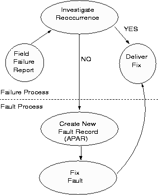
Figure 1: Fault and Failure Process
Using Service Process data holds much promise. There are two independent reasons that motivate this direction. First, the service process reaches out to the entire customer base. Second, this data is actively used to manage the business and product development. This latter point is an important link to recognize and exploit. Given that the failures in the field are caused by faults in the software which are ultimately fixed by development, the quality of the data is eminently better. Development organizations tend to carefully account for faults in the product, but may not care too much about tracking the failure process. On the other hand, the Service organizations do track the failures and repairs closely. Between the two, often disparate sources of data, there is a significant opportunity for the measurement of commercial software failure rates. Since failures are reported across the entire customer base of the product, there is far greater coverage of failure events experienced on the product. Although there would be substantial under-reporting, it is still a much more representative event space than carefully studying a small subset of machines or customers accounts. To reasonably represent the entire customer set, it is necessary to use a large sample (at least several hundreds), if not the entire population. Even when the data is available, the challenge is to be able to use it, which is no simple task.
Data
To use this data, one has to understand the subprocesses of faults and failures, to extract the right measurements and devise appropriate filter mechanisms for the data. Figure 1 illustrates a state transition diagram showing the key events relevant to us. The reason we describe both the failure process and the fault process is to provide a clear understanding of the service process and gain insight on data available. When a customer has a problem with a software product, they can call the customer support service. This facility is available for all kinds of problems customers may face. The problems can include failures due to software, requests for how-to information, installation etc. etc. Most calls do not relate to software failure. There are however, a small fraction of calls that are software failures, resulting from defect oriented problems, which is the focus of this paper.
When a failure is reported and identified as a potential code related failure, a problem record is created and an investigation begins. The investigation searches the failure data base to see whether the problem is known and a fix is readily available. If the investigation yields an immediate solution, namely the rediscovery of a known fault, the fix is dispatched and it terminates the failure tracking cycle. Sometimes, after investigation, it is determined that the failure corresponds to a new fault being reported. In this case, a new fault report is initiated, which in IBM parlance is called the Authorized Program Analysis Report, (APAR). The failure tracking process is not yet completed and waits for the fault process to complete. A change team fixes the fault and makes the fix available to the service team, and also documents its characteristics so that future failures due to this fault can be easily recognized. Change teams sometimes exist within the development organization, following their practices of tracking defects. A more detailed description of the service process can be seen in [CRGR93] and [SC91].
Not every fault is experienced by each customer; in fact there are several faults that are reported only once. This is due to the peculiarities of an environment that triggers a failure. Customers have access to all fixes for known faults. Usually at periodic intervals, customers upgrade their software to include all known fixes. On the other hand, several customers do not want to fix what is not broken, and are very selective in applying fixes. Some faults, however, are considered highly pervasive by the service team, which urges customers to install these fixes as soon as possible.
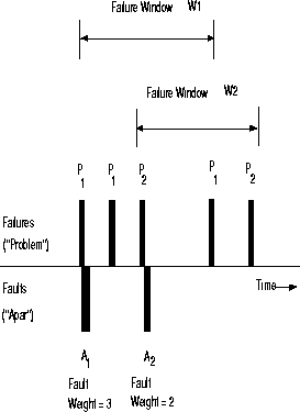
Figure 2: Time line of Failures and Faults
Figure 2 shows the impact of different faults and failures as they would appear on a time line across the entire customer base. Failures and Faults are shown on the time line, on the upper and lower sides respectively. A vertical bar above the line represents a failure, and the one below, a fault. The very first time a failure (IBM term, Problem) is reported it would cause the creation of new fault record (APAR) to address the failure. In the figure, P1 represents the failure which causes the identification of new fault A1. Subsequently there can be multiple occurrences of the failure P1 which would not require creation of an APAR. Instead, the repair for the failure P1 is available to the customers and soon the investigation figures out that the failure corresponds to the fault A1. Failures P1 and P2 re-occur in the customer base at different customer sites and are shown with repeated occurrences along the time line.
Failure/Fault Relationship
One might wonder, why bother with faults, when we are interested in failure rate? The issue is one of identifying the right subset of all reported failures of a product, to just those that are due to the product. When a defect oriented problem call comes in, it is routed to a team that knows the family of products. However, it is not immediately evident which of the numerous software products caused the failure. It could be that the failure is manifested in one product, whereas the failure actually occurs at a layer below in another product, (e.g. the operating system), or in a peer middleware software product with which the incident product shares resources. Therefore, before we start counting failures to measure failure rates, we need to identify the right subset of failures that pertain to the product under study. Establishing the link with the fault in the product is an unequivocal way to make certain the failure is related to the specific product in question. This is because the fault record (APAR) ultimately identifies the line(s) of code that causes the failure.
Establishing the link between the fault and failure is a simple concept in theory but a complicated task in practice. There are several issues that need to be grappled with. We were fortunate to be able to do so with the available data. It involved not only a clear understanding of the content of disparate databases, but also a detailed set of interviews with service personnel. Essentially, we needed to understand their practices of recording data, and the idiosyncrasies of the Problem and APAR tracking systems. To illustrate a few of the challenges: Failures and faults are tracked separately and handled by different segments of the service process. We found that data about a fault did not generally exist in the failure record initially, however, it did when the problem was resolved. Where was it and was it consistently retrievable? We found that the fault was tagged in the failure record for the product. This was a significant step forward, because it meant that we would be able to extract reasonably accurate data. Another issue, that is not apparent to the casual observer is the sheer volume of failure data that needs to be processed. Failure data involves a significant amount of dialog back and forth between the customer and the service person, and is therefore voluminous. Given the size, most of it is not saved and is deleted periodically. A subset of the data, with key fields are selectively archived. This data, from a family of products across world wide service needs to be processed against the fault data to identify the failures due to the product. Once we extract the failures using the faults in the product, we have the necessary event stream to compute failure rates.
Given the event sequence of failures and faults, across the customer base, we have an opportunity to learn more about this process. To describe and understand the fault and failure processes we define two metrics: failure window and fault weight.
The failure window is the length of time between the first and last known occurrence of a failure from a specific fault. In figure 2, the periods of time W1 and W2 are the failure windows for faults A1 and A2 respectively. Essentially, each fault has a non zero failure window, if it ever reappeared in the customer base. The last occurrence is clearly dependent on the observation period, and like all real failure data, is right censored. The fault weight is the number of failures resulting from a fault. In other words, it is the number of failures that are observed during its failure window. In this example, the fault A1 has a weight of 3 and the fault A2 has a weight of 2. Extending the time interval for observation could result in a longer failure window and larger fault weight for a given fault.
The failure window should not be confused with the grouping of error events, occuring within a short interval of time, into tuples [TS83, LS90, IYS86]. The use of tuples is primarily to group a burst of errors that occurs into one logical failure event. This coalescing process is done on errors, occuring on the same machine, since they are most likely related to each other. The failure window is a different measure from such coalescence time periods, being defined on failures occurring on different systems and possibly different customer accounts, over prolonged periods of time. The window is defined on failures appearing across the entire install base, whereas the previous efforts focused on multiple failures reported on a single system. Usually when a problem is reported via the service process, the human has already coalesced any multiple error conditions into one logical failure. Thus the failures we analyze are already coalesced.
The two measures, fault weight and failure window are natural to the fault and failure process. The purpose of describing them is not for measurement of the failure rate from observed data. The failure rate can be estimated without the use of these metrics. However, these metrics provide the intuition to understand the failure process better. We will, therefore, provide statistics of fault weight and failure window. The fault weight is an indicator of the frequency or rareness of a failure resulting from a given fault. The failure window suggests the length of exposure from a particular fault, and provides a measure of dispersion of the failures resulting from a given fault. Together, they provide us with significant insight into the composition of the overall failure rate. One advantage of the weight and window metrics is that it opens the possibility of constructing better reliability models. In this paper, we do not pursue that, but lay the foundation by providing the statistics of these metrics. The paper of [Ada84] is an example of such an effort, but does not get into the concept of failure window. It does divide faults into different classes based on failure rates, thereby indirectly using a weight like metric.
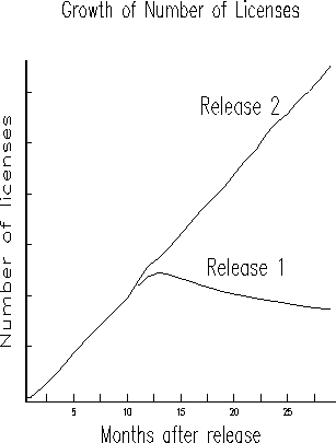
Figure 3: License Base in the Field
An important ingredient to the computation of the failure rate of software is the install base in the field. Fortunately, this data is usually well tracked given that it has to do with product revenue. The computation of install base considers, existing licences, new licences, and migration from old releases into new releases. Figure 3 shows how these curves may look. Usually, sales of new computers occur with the latest release of software, and there is also a migration from the earlier release to the new one. This data is used to normalize the failure rate to a per machine basis.
Another factor that needs to be compensated for is the under-reporting of problems into the service center. Under-reporting is a function of the way customers deal with problems and the services and system management associated with their system. The number of problems reported into the service process is only a fraction of what occurs in the field. Through customer surveys and interviews with people knowledgeable in service, we believe that the under-reporting is between 80 to 90 percent. This translates to a failure rate, which is about 5 to 10 times of what is reported. For this paper, we will use a factor of 10 to scale up the reported failure rate to arrive at the adjusted failure rate. Since we only have a rough estimate of the level of under-reporting, we can only assert that our scaled failure rate is within an order of magnitude of the actual failure rate. We do not attempt to assign a confidence level to this claim, since there is no objective basis for doing so. Given how little is known about real failure rates for commercial software, getting an order of magnitude estimate is, we believe, a significant achievement.
Results
Once we have the failure events per month, the license base and the under-reporting factors, we can compute the failure rate on a per machine-month basis. Figure 4 shows the overall reported failure rates of two releases of software - superimposed on each other, unadjusted for under-reporting. The time axis for each has been positioned to reflect months after release into the field. The ordinate is in units of failures per machine per month. For release 1, the graph shows only the data starting from around month 10. Earlier data was unavailable in the database. It may be safe to presume that the failure rate for earlier months is higher.
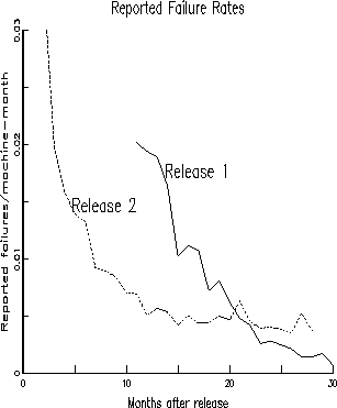
Figure 4: Software Failure Rates of Release 1 and 2
We observe that, about three months after the release, the failure rate for release 2, adjusted for under-reporting, is around 0.2  , while release 1 achieved the same level after about 10 months in the field. We also observe that the failure rate for Release 2 has come down rapidly in the first year in the field and has been decreasing more slowly since. On the other hand, for release 1, the failure rate has started from a presumable higher level and has continued to drop rapidly over a longer period. About 21 months after the general availability date, the failure rate for Release 1 is less than that of release 2 after the same duration in the field. The continued rapid drop for Release 1 may be partly due to less support for the older release, following the availability of the new release. It may also be presumed that the users remaining with release 1 are the ones experiencing fewer major problems.
The failure rates, adjusted for underreporting, when plateaued, are around .02 per machine per month for Release 1 and around .04 for release 2, corresponding to mean times between failures of about 4 years and 2 years, respectively. These numbers provide one of the first order of magnitude estimates for perceived failure rates of widely used operating systems. The high MTBF for Release 1 was attained only after being in the field for over 3 years.
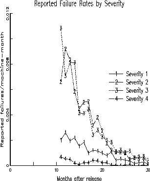
Figure 5: Failure Rate by Severity - Release 1
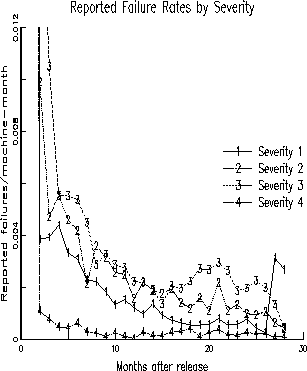
Figure 6: Failure Rate by Severity - Release 2
The failure rate that is shown in the earlier figure is the combination of failures of different severity classes. In IBM, each failure (and the underlying fault) is categorized into severity 1, 2, 3, or 4 which represent decreasing degrees of severity. Severity 1 usually implies a failure that disables every application on the operating system. Severity 2 implies a serious, but not catastrophic disruption of work. Severity 3 and 4 are much less severe failures that would usually be considered annoyances. In the next two figures, we divide the overall failure rate into that contributed by the different severity classes. Figures 5 and 6 show the failure rates of releases 1 and 2 (unadjusted for underreporting), separated by the different severity classes. It is evident that the severity 1 failures are much lower than severities 2 and 3. Failures of all severities follow roughly the same decreasing trend as a function of time.
Fault Weight and Failure Window
The fault weight and failure window provide us with intuitive metrics to understand the failure process that ensues in the field. The fault weight, defined in section 2, is a measure of the impact of a fault on the overall failure rate. The failure window, on the other hand, measures the dispersion of that impact over time. For a given observation period, and a fixed fault weight, a smaller failure window implies a more rapidly decreasing failure rate than a larger failure window.
Essentially, these are two orthogonal measurements on the failure process. Together, they provide an insight into a failure process. Understanding their statistics can be useful to glean the mechanics taking place in the field. Table 3.1 shows mean values of several metrics including the fault weight and failure window, by severity and release. For each severity and release, the table shows the number of faults in that class, the mean fault weight, and the mean failure window. Also shown is the proportion of faults with weight greater than one. Note that a nontrivial failure window is defined only if there are two or more failures for a given fault. This probability describes the fraction of faults for which a window exists. The last row shows the average of the ratios of the failure window to the fault weight, for faults with more than one failure. (Note that it is not the simple division of row 2 and 1).
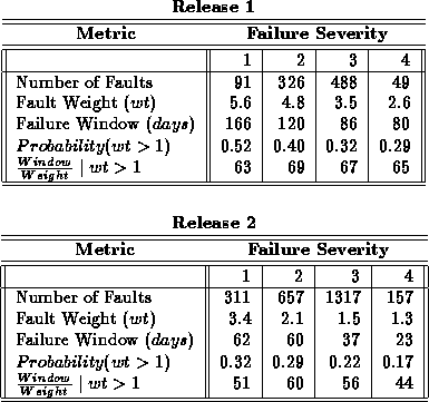
Table 1: Average Fault Metrics by Severity
There are several points that can be gleaned about the failure process, from these metrics.
First, notice that the fault weights are decreasing with severity in both releases. Severity 1 is the highest and 4 the least. The severity of the fault (and also the failure) is determined purely by the judgment of the customer and the service personnel. To a large extent severity is a qualitative assessment. Thus, it is interesting to see that the higher severity faults do have a higher fault weight, consistently across all 4 severities. This is true for both releases although the fault weights themselves change between the releases.
Second, the same is true for failure windows. The mean failure window, for severity 1 to 4, goes from 166 days down to 80 days for release 1, and from 62 days to 23 in release 2. This shows that a higher severity fault tends to cause more failures, and for longer periods of time than a low severity fault.
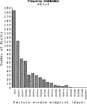
Figure 7: Distribution of Failure Windows for release 2
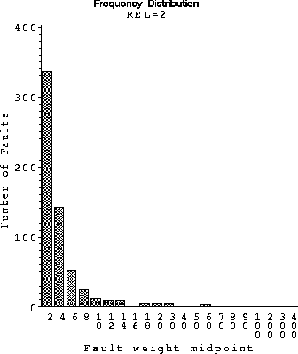
Figure 8: Distribution of Fault Weights for release 2
Third, the majority of the failures in almost all categories occur only once. This is evident from the column of probability of weight greater than 1, where most values are less than half. Also, the proportion of failures that do repeat decreases with severity. This implies that the higher severity faults are more likely to cause multiple failures. This is consistent with the observations on the mean fault weight, and would be expected intuitively. The overall proportion of faults that cause multiple failures is 36 percent for release 1 and 25 percent for release 2. On the other hand, the proportion of failures that are re-occurrences (due to the same fault) is 76 percent for release 1 and 47 percent for release 2. These may be compared with the 72 percent reoccurrence proportion reported in [LI93].
Finally, the last column is the average of the failure window divided by the fault weight for faults with weight greater than one. The units of this would be days per failure. It is interesting to see that this measure is unrelated to severity. Although the magnitudes differ by release, they are almost the same within a release. This final observation suggests that the fault weight and failure window metrics could be useful for a more detailed modelling of the failure process. We have confirmed, based on regression analysis tests, that the differences in average window/weight ratio between different severity classes are not statistically significant, for either release, while the other metrics do differ significantly, for both releases. (All of these observations hold for any significance level from .10 to .001).
In the interest of providing potential areas for further investigation, we show the distributions of the fault weight and failure window from Release 2 in Figure 7 and 8. The distributions for release 1 show similar patterns. We have empirically observed that the fault weights follow the Zipf-Estoup law [JK69], more commonly known as the Zipf's law. This has been also used in various other applications, especially the distribution of word frequencies [Goo57]. The failure windows fit a Weibull distribution.
Summary
This paper addresses a critical need in the fault tolerant computing area of today. As commercial software is distributed to hundreds of thousands of customers, and studies point to software as a significant contributor to outage and failure, measuring the actual failure rate perceived by an end user becomes critical. This one parameter has a significant influence on the overall design for dependability. It has been an elusive parameter to measure, with several indirect methods proposed, and despite the focus, with little data available. Sadly, experts grope even for an order of magnitude measure for the failure rate of such commercial software.
This paper address the above need and provides quantitative results. The study is conducted on two releases of a software product (with several million lines of code) distributed to a large customers base. The key difference between this study and several others is that we use failures reported into the service process, from a world wide customer base, to directly measure failure rate. This, however, is not an easy task. To isolate just those software failures belonging to a product, we tie each reported failure to the fault that caused it, so that it can be traced to the specific product. This technique yields, to the best of our knowledge, some of the finest measurements for a commercial software product. It also allows us to provide very detailed quantified results. Among some of them reported are:
- The failure rates of Release 1 and Release 2 of this product plateau at about 0.02 and 0.04 failures per machine-month, respectively. The plateaus occur around 3 years and 18 months after the respective release dates. To a first order of approximation, they correspond to MTBFs of 4 years and 2 years. We also present the change in failure rate as a function of time, release, and severity. The order of magnitude measures would be eye openers for the industry.
- The fault weight, (number of failures due to a fault), of the higher severity faults tends to be higher than that for the lower severity faults. This may sound intuitive and obvious, but for the fact that the assignment of severity is an entirely qualitative judgment based on customer feelings and service representative's opinion. A similar trend is noted for the failure window, (length of time between the first and last occurrence of failures for a particular fault). The windows are larger for the higher severity faults. These trends are systematic between all severities and releases.
- The failure window and fault weight provide natural and intuitive measurements of the failure process. The fault weight measures the impact of a fault on the overall failure rate. The failure window on the other hand measures the dispersion of that impact over time. These metrics provide a new forum for discussion and an opportunity to better model, understand and possibly control the failure process across a customer base.
This paper should be of interest to all working in the area of fault tolerance of systems that contain software.
References
Edward Adams. Optimizing Preventive Service of Software Products. IBM Journal of Research and Development, 1984.
M. J. Buckley. Computer Event Monitoring and Analysis. In Ph.D. Thesis, Carnegie Mellon University, 1993.
R. Chillarege. Top 5 challenges facing the practice of fault-tolerant computing. Lecture Notes in Computer Science, 774, Hardware and Software Architectures for Fault Tolerance, Springer-Verlag, 1994.
R. Chillarege, B. K. Ray, A. Garrigan, and D. Ruth. Software recreate problem estimated to range between 10-20 percent: A case study on two operating system products. Proceedings, Fourth International Symposium on Software Reliability Engineering, 1993.
X. Castillo and D. Siewiorek. A Workload Dependent Software Reliability Prediction Model. Digest of Papers The 12th International Symposium on Fault Tolerant Computing, pages 279-286, 1982.
R. Cramp, M. A. Vouk, and W. Jones. On Operational Availability of a Large Software-Based Telecommunication System. Third International Symposium on Software Reliability Engineering, 1992.
I. J. Good. Distribution of Word Frequencies. Nature, 1957.
J. Gray. A Census of Tandem System Availability between 1985 and 1990. IEEE Transactions on Reliability, 39(4):409-418, Oct 1990.
R. Iyer and P. Velardi. Hardware Related Software Error: Measurements and Analysis. IEEE Transactions on Software Engineering, SE-11(2), Feb 1985.
R. K. Iyer, L.T. Young, and V. Sridhar. Recognition of Error Symptoms in Large Systems. In Proceedings of Fall Joint Computer Conference, 1986.
N. L. Johnson and S. Kotz. Discrete Distributions. Houghton Mifflin Company, 1969.
G. Q. Kenney. Estimating Defects in Commercial Software During Operational Use. IEEE Transactions on Reliability, March 1993.
K. Kanoun and T. Sabourin. Software Dependability of a Telephone Switching System. Digest of Papers The 17th International Symposium on Fault Tolerant Computing, 1987.
G. Q. Kenney and M. A. Vouk. Measuring the Field Quality of Wide-Distributed Commercial Software. Proceedings, Third International Symposium on Software Reliability Engineering, 1992.
J. C. Laprie. Dependability: Basic Concepts and Terminology. Dependable Computing and Fault-Tolerant Systems, Springer-Verlag, 5, 1992.
I. Lee and R. K. Iyer. Faults, Symptoms, and Software Fault Tolerance in the Tandem GAURDIAN90 Operating System. In Digest of Papers The 23rd International Symposium on Fault-Tolerant Computing, pages 20-29, 1993.
I. Lee, R. K. Iyer, and A. Mehta. Identifying Software Problems Using Symptoms. In Digest of Papers The 23rd International Symposium on Fault-Tolerant Computing, pages 20-29, 1993.
T. Lin and D. Siewiorek. Error Log Analysis: Statistical Modelling and Heuristic Trend Analysis. IEEE Transactions on Reliability, 39(4):419-432, October 1990.
S. Mourad and D. Andrews. On the Reliability of the IBM MVS/XA Operating System. IEEE Transactions on Software Engineering, SE-13:1135-1139, 1987.
M. Sullivan and R. Chillarege. Software Defects and their Impact on System Availability - a study of Field Failures in Operating Systems. In Digest of Papers The 21st International Symposium on Fault-Tolerant Computing, pages 2-9, 1991.
M. M. Tsao and D. Siewiorek. Trend Analysis on System Error Files. In Digest of Papers The 13th International Symposium on Fault-Tolerant Computing, 1983.